O1 (WP1) – The theory of transport and machine learning architectures
Deliverable: A comprehensive turbulent transport model
Within this work package, we established the theoretical foundations for describing the dynamics of charged particles in fusion plasmas characterized by turbulence (Task 1.1), for the correct description of turbulent random fields (Task 1.2), and for the main machine-learning tools relevant to the purpose of this project (Task 1.3).
We consider a population of charged particles, with mass $m$ and charge $q$, confined in a tokamak configuration dominated by a strong magnetic field $\mathbf{B}$. The usual particle coordinates in phase space are $(\mathbf{x},\mathbf{v})$. When the magnetic field is sufficiently strong compared to other electromagnetic components, the motion can be viewed as a superposition of a smooth large-scale motion and a fast Larmor gyration. This scale separation is the basis of Lie perturbation theory [1], which provides a rigorous mathematical framework for charged-particle dynamics in magnetized plasmas.
In this approach, the true 6D phase space $(\mathbf{x},\mathbf{v})$ is replaced by the reduced gyrocentre coordinates $(\mathbf{X},v_{\parallel},\mu)$, which suppress the fast gyromotion through a perturbative expansion based on gyrokinetic ordering [2]. In this project we adopt the high-flow ordering [3], explicitly retaining the polarization drift [4].
The gyrocentre dynamics satisfy
$$ \frac{d\mathbf{X}}{dt} = v_{\parallel}\frac{\mathbf{B}^\star}{B_{\parallel}^\star} + \frac{\mathbf{E}^\star \times \mathbf{b}}{B_{\parallel}^\star} \qquad\text{(1)} $$
$$ \frac{dv_{\parallel}}{dt} = \frac{q}{m}\frac{\mathbf{E}^\star\cdot\mathbf{B}^\star}{B_{\parallel}^\star} \qquad\text{(2)} $$
$$ \frac{d\mu}{dt}=0 \qquad\text{(3)} $$
where $$\mathbf{E}^\star = -\nabla\Phi^\star - \frac{\partial \mathbf{A}^\star}{\partial t}, \qquad \mathbf{B}^\star = \nabla\times\mathbf{A}^\star,$$ and
$$ q\Phi^\star = \frac{m v_\parallel^2}{2} - \frac{m u^2}{2} + \mu B + q\phi_1^{\text{neo}} + q\phi_1^{\text{gc}} \qquad\text{(4)} $$
$$ \mathbf{A}^\star = \mathbf{A}_0 + \frac{m}{q}(v_{\parallel}\mathbf{b}+u+v_E) + \mathbf{A}_1^{\text{gc}} \qquad\text{(5)} $$
The zeroth-order magnetic potential $\mathbf{A}_0$ satisfies $\mathbf{B} = \nabla\times\mathbf{A}_0$. For axisymmetric equilibria, the field can be written as: $$ \mathbf{B} = F(\psi)\nabla\phi+\nabla\phi\times\nabla\psi, $$ where $\phi$ is the toroidal angle in cylindrical $(R,Z,\phi)$ or toroidal $(r,\theta,\phi)$ coordinates (COCOS = 2) [5].
The local safety factor $q_\theta(\psi,\theta)$, its flux-surface average $\bar{q}(\psi)$, and the generalized poloidal angle $\chi(\psi,\theta)$ are defined by:
$$ q_\theta(\psi,\theta) = \frac{\mathbf{B}\cdot\nabla\phi}{\mathbf{B}\cdot\nabla\theta} \qquad\text{(6)} $$
$$ \bar{q}(\psi) = \frac{1}{2\pi}\int_0^{2\pi} q_\theta(\psi,\theta)\,d\theta \qquad\text{(7)} $$
$$ \left.\frac{\partial\chi}{\partial\theta}\right|_{\psi} = \frac{q_\theta(\psi,\theta)}{\bar{q}(\psi)} \qquad\text{(8)} $$
Zeroth-order MHD equilibrium is toroidally invariant and constant on magnetic surfaces, so $n=n(\psi)$, $P=P(\psi)$, $T_i=T_i(\psi)$, $T_e=T_e(\psi)$.
A macroscopic radial electric field $E_0$ produces a toroidal rotation $$ \mathbf{u} = R^2\Omega_t(\psi)\,\nabla\phi, $$ where $\Omega_t(\psi)$ may have a gradient. The equations of motion are expressed in a frame rotating with $\mathbf{u}$ [3,7]. Poloidal flows are neglected [5], but a neoclassical poloidal potential $\phi_1^{\text{neo}}(\psi,\theta)$ appears:
$$ \phi_1^{\text{neo}} = \frac{m\Omega_t(\psi)^2}{2|e|\,(1+T_i/T_e)} \left(R^2 - \langle R^2\rangle_\theta\right) \qquad\text{(9)} $$
The first-order gyrocentre potentials $\phi_1^{\text{gc}}$ and $\mathbf{A}_1^{\text{gc}}$ include turbulent fluctuations and small external perturbations (RMPs). Gyro-averaging gives:
$$ \tilde{\phi}_1^{\text{gc}}(k,t) = \tilde{\phi}_1(k,t)\, J_0(k_\perp \rho_L), $$ with $\rho_L=\sqrt{2m\mu}/(qB)$.
The drift-wave turbulence relevant for ions is dominated by ITG/TEM modes [8].
Circular geometry
In circular approximation, $$ \mathbf{B} = B_0 R_0\,\nabla\phi + \frac{r b_\theta(r)}{R}\,\nabla\theta \qquad\text{(10)} $$ $$ F(\psi)=B_0 R_0 \qquad\text{(11)} $$ $$ \psi(r)=B_0R_0\int_0^r b_\theta(r')dr' \qquad\text{(12)} $$ $$ b_\theta(r)=\frac{r\,\bar{q}(r)}{R_0^2-r^2} \qquad\text{(13)} $$ $$ \chi(r,\theta)=2\tan^{-1} \left[\frac{R_0-r}{R_0+r}\tan\left(\frac{\theta}{2}\right)\right] \qquad\text{(14)} $$
Solov’ev equilibria
With linear profiles: $$ \mu_0\frac{dP}{d\psi}=A, \qquad \frac{dF^2}{d\psi}=\frac{2 A R_0^2 \gamma}{1+\alpha^2} \qquad\text{(15)} $$ The poloidal flux is $$ \psi=\frac{A}{2(1+\alpha^2)} \left[R^2 - \gamma R_0^2 - Z^2 + \frac{\alpha^2}{4}(R^2-R_0^2)^2\right] \qquad\text{(16)} $$ Minor radius: $$ a=\frac{R_0}{2\sqrt{2-\gamma-\sqrt{\gamma}}} \qquad\text{(17)} $$ Elongation: $$ \kappa=\frac{\alpha}{\sqrt{1-\gamma/(2-\gamma)}} \qquad\text{(18)} $$ Current: $$ F(\psi)=B_0R_0\left[1+\frac{\psi}{2A\gamma B_0(1+\alpha^2)}\right] \qquad\text{(19)} $$
Experimentally reconstructed equilibria
Experimental magnetic equilibria (G-EQDSK format) provide $\psi(R,Z)$ and profiles $F(\psi)$, $\bar{q}(\psi)$ on numerical grids. They are generated by reconstruction tools such as CHEASE [9], EFIT [10], PLEQUE [11], NICE [12], and EQUINOX [13]. T3ST uses these equilibria when analyzing specific discharges.
Given the definitions of the magnetic equilibrium quantities $q_\theta(\psi,\theta)$, $\bar{q}(\psi)$, and $\chi(\psi,\theta)$ (Eqs. (6–8)), one can show that the Clebsch form of the magnetic field is valid:
$$ \mathbf{B} = \nabla(\phi - \bar{q}\,\chi)\times\nabla\psi. $$
For representing small-scale turbulent fluctuations, most gyrokinetic (GK) codes adopt field-aligned coordinates $(x,y,z)$ [14], which simplify the description of fluctuations elongated along magnetic field lines. These coordinates correspond to the radial, binormal, and parallel directions ($\mathbf{B}\propto\nabla y\times\nabla x\propto\partial \mathbf{r}/\partial z$):
$$ x = C_x f(\psi) \qquad\text{(20)} $$
$$ y = C_y\,( \phi - \bar{q}\,\chi ) \qquad\text{(21)} $$
$$ z = C_z\,\chi \qquad\text{(22)} $$
In practice, T3ST uses constant values $C_x=a$ (the tokamak minor radius), $C_y=r_0/\bar{q}(r_0)$ (with $r_0$ a reference radius), $C_z=1$, and defines $f(\psi)=\rho_t = \Phi_t(\psi)/\Phi_t(\psi_{\text{edge}})$, where $\rho_t\in[0,1]$ is the normalized effective radius. The toroidal magnetic flux is
$$ \Phi_t(\psi)=\int_{\text{axis}}^{\psi} \mathbf{B}\cdot\mathbf{e}_\phi\, dS(\psi'), $$
thus $\rho_t \approx r/a$ (in circular geometry).
Instead of computing turbulent fields self-consistently, T3ST models them statistically as an ensemble of random fields $\{\phi_1, A_1\}$ with prescribed statistical properties, consistent with experimental ITG/TEM observations. Several moderate assumptions are used:
-
Gaussianity — Fluctuations are assumed to follow a normal distribution $P[\phi_1]\sim\exp(-\phi_1^2/2\langle\phi_1^2\rangle)$. Small experimental deviations from Gaussianity have negligible impact on transport.
-
Homogeneity — Turbulence is taken as homogeneous. Thus the autocorrelation function $$ E(\mathbf{r},t;\mathbf{r}',t') = \langle \phi(\mathbf{r},t)\phi(\mathbf{r}',t')\rangle = E(\mathbf{r}-\mathbf{r}',\,t-t') $$ contains all statistical information and can be evaluated from the power spectrum $S(\mathbf{k},\omega)=\langle|\tilde{\phi}_1(\mathbf{k},\omega)|^2\rangle$.
-
Drift-type dispersion relation — ITG/TEM fluctuations originate from drift-wave instabilities described approximately even in the saturated state by a dispersion relation $\omega^\star(\mathbf{k})$. In the code: $$ \omega^\star(\mathbf{k}) = \frac{\mathbf{k}\cdot\mathbf{V}^\star}{1+\rho_s^2\,|\mathbf{k}_\perp|^2}, $$ where $\mathbf{V}^\star = -(\nabla p_s\times\mathbf{b})/(n_s q_s B)$ is the diamagnetic velocity of species $s$, and $\rho_s$ is its Larmor radius.
Based on these assumptions, T3ST constructs an ensemble of random fields $\phi_1(x,t)$ from white-noise fields in Fourier space $\eta(\mathbf{k},\omega)$ satisfying $$ \langle \eta(\mathbf{k},\omega)\,\eta(\mathbf{k}',\omega')\rangle = \delta(\mathbf{k}+\mathbf{k}')\,\delta(\omega+\omega'). $$ The Fourier components of the potential are
$$ \tilde{\phi}_1(\mathbf{k},\omega) = \sqrt{S(\mathbf{k},\omega)}\,\eta(\mathbf{k},\omega), $$
ensuring Gaussianity and correct correlations.
In toroidal geometry, the fields can be expressed through a double Fourier series:
$$ \phi(x,t)=\sum_{n,m}\phi_{nm}(r,t)\, e^{i(n\phi+m\theta)} \qquad\text{(23)} $$
which preserves natural periodicity. However, due to the anisotropic nature of turbulence (long correlation lengths along the field, short perpendicular), field-aligned representation is preferred. Thus T3ST evaluates $\phi_1$ in field-aligned coordinates, even though magnetic drifts are computed in cylindrical coordinates.
The random field is represented as:
$$ \phi_1(x,y,z,t) =\int dk\, d\omega\; \tilde{\phi}_1(\mathbf{k},\omega)\; e^{\,i(k_x x + k_y y + k_z z - [\omega^\star(\mathbf{k})+\omega] t)} \qquad\text{(24)} $$
For $k_\parallel\ll k_\perp$, the correspondence with toroidal mode numbers is approximately:
$$ k_y \approx \frac{n}{C_y},\qquad m = -\big[\bar{q}(x_0)\,n\big] + \Delta m,\qquad k_z = \frac{\Delta m + \{\bar{q}(x_0)n\}}{C_z}, \qquad\text{(25)} $$
where $[\cdot]$ and $\{\cdot\}$ denote the integer and fractional parts, and $n,\Delta m\in\mathbb{Z}$.
The spectrum $S(\mathbf{k},\omega)$ is modeled analytically to reproduce saturated drift-wave turbulence characteristics:
$$ S = A_\phi^2 \, \frac{\tau_c\,\lambda_x\lambda_y\lambda_z}{(2\pi)^{5/2}}\, \frac{ \exp\!\left[-(k_x^2\lambda_x^2 + k_z^2\lambda_z^2)/2\right] }{ 1+\tau_c^2\omega^2 }\, \Big[ e^{-\frac{(k_y-k_0)^2\lambda_y^2}{2}} \;-\; e^{-\frac{(k_y+k_0)^2\lambda_y^2}{2}} \Big] \qquad\text{(26)} $$
The parameters $\lambda_x,\lambda_y,\lambda_z$ are the correlation lengths in the field-aligned directions; $k_0$ selects the most unstable mode $$ k_{y,\text{max}} \approx \frac{k_0}{2} + \sqrt{\frac{k_0^2}{4} + \frac{2}{\lambda_y^2}}. $$ The correlation time $\tau_c$ measures deviations from the dispersion relation, and $A_\phi$ sets the turbulence amplitude. Typical parameters:
$$ \lambda_x \approx 5\rho_i,\quad k_0 \approx 0.1/\rho_i,\quad \lambda_y \approx 5\rho_i,\quad \lambda_z \approx 1,\quad \tau_c \approx R_0/v_{\text{th}},\quad |e|A_\phi \approx 1\%\,T_i. $$
Since $\lambda_z\approx 1$, we obtain $\lambda_\parallel\approx\bar{q}R_0$, consistent with experimental observations.
Drift-wave turbulence in tokamaks is generally a superposition of ITG and TEM modes, weighted by coefficients $A_i$ and $A_e$:
$$ \phi_1 = A_i\,\phi_1^{\text{ITG}} + A_e\,\phi_1^{\text{TEM}}, \qquad A_i + A_e = 1. $$
It is well known that magnetic curvature, shear, internal transport barriers, ELM activity, and blob structures can induce non-Gaussian behavior and spatial variations of turbulence. Thus the assumptions of Gaussianity and homogeneity are only approximate. Nevertheless, numerical results (Sec. 4) show that particle transport is predominantly local, with particles moving only a few Larmor radii from their initial surface. Therefore, although not globally exact, these assumptions remain valid locally for the purposes of the present analysis.
A possible extension recently implemented in the T3ST code is the ability to include inhomogeneities along the direction parallel to the magnetic field (“z”) through a simple prefactor:
$$ \phi_1 \rightarrow \phi_1 \, g(z) $$
$$ g(z) = e^{-\, z^2 / (2 \Lambda_z^2)} $$
where \( \Lambda_z \) is a measure of the parallel correlation and of the “ballooning” character specific to electrostatic turbulence.
Let an arbitrary function be \(F(\mathbf{X}) = y\), where \(\mathbf{X}\) is the “input” vector of size \(\mathbf{X}\in\mathbb{R}^{N}\), and \(y\) is the “output” which, in our case, is a scalar \(y\in\mathbb{R}\). Machine-learning models are designed to approximate complex relationships between input–output pairs, i.e. mappings \(\mathbf{X}\mapsto y\), especially when the analytical form of the function is unknown, difficult to derive, or impossible to reproduce explicitly.
In the context of this project, the objective is to predict the asymptotic diffusion and convection values as functions of the free parameters of the transport model. These free parameters can be grouped into three categories: parameters describing the plasma equilibrium profiles, parameters of the particle distribution under consideration, and turbulence parameters. In total, depending on the available information, the asymptotic diffusion may depend on approximately 20 independent variables, so that the input vector has dimension \(\mathbf{X}\in\mathbb{R}^{20}\).
The main obstacle to achieving accurate predictions comes from the high complexity of the multivariate function, driven by the large dimensionality of the input space. Moreover, this difficulty is amplified by the limited size of the training database, which cannot be expanded arbitrarily due to the computational cost of the numerical simulations.
In this setting, it is necessary to identify machine-learning methods—combined with sampling and preprocessing techniques—that provide good performance in high-dimensional spaces and adapt efficiently to small datasets. For such problems, the most suitable models are nonlinear regression methods, in particular feed-forward neural networks (NNs) [15], which are universal approximators and can capture complex nonlinear relationships in continuous high-dimensional functions. Complementarily, dimensionality reduction techniques such as PCA [16] can be used to extract relevant features and reduce the NN input space, improving both stability and predictive accuracy.
In essence, a neural network is a function with a specific structure that maps an input of dimension \(d_0\) to an output of dimension \(d_{n+1}\). The basic structure is composed of layers of three types: an input layer (\(L_0 \equiv L_{\text{in}}\)), an output layer (\(L_{n+1} \equiv L_{\text{out}}\)), and, between them, one or more “hidden” layers (\(L_i\), \(i=\overline{1,n}\)). The basic elements of each layer are neurons, and their number may vary from layer to layer (denoted by \(d_i\)).
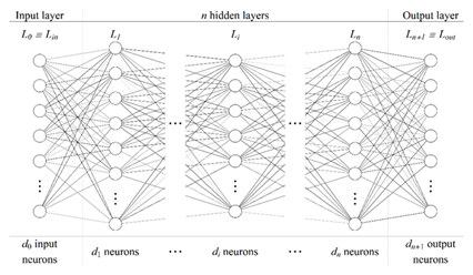
For the problem analyzed in this project, the most appropriate neural-network model is a fully connected feed-forward neural network (FCNN) [16]. In such an architecture, each neuron in a layer is connected to all neurons in the next layer, and information propagates unidirectionally from input to output through one or more hidden layers. A generic FCNN architecture is illustrated schematically in Figure 1.
The inputs and outputs of an NN must be numerically quantifiable, so that each neuron represents a single numerical value. In the present study, the input is the set of \(\sim 20\) free parameters of the transport model, and the output is the scalar value of the asymptotic radial diffusion.
Equation (1.22) describes how the value of a generic neuron, denoted \(\alpha^{(i)}_j\), is computed. This quantity represents the value of the \(i\)-th neuron in layer \(L_j\):
where:
- \(w^{(i,k)}_j\) is the weight assigned to the value of the \(k\)-th neuron in the previous layer (\(L_{j-1}\));
- \(f\) is the activation function, which can take various forms; commonly used choices are sigmoid or the hyperbolic tangent (\(\tanh\)). One of its roles is to introduce nonlinearity into an otherwise linear combination of weights and neuron values (a weighted sum over the \(d_{j-1}\) neurons of layer \(L_{j-1}\));
- \(\beta^{(i)}_j\) is the bias associated with neuron \(i\) in layer \(L_j\), whose role is to shift the input range of the activation function.
In matrix notation, the compact form of Eq. (1.22) for the entire layer \(L_j\) is:
Here \(\mathbf{A}_j\) and \(\mathbf{A}_{j-1}\) are column vectors of sizes \(d_j\times 1\) and \(d_{j-1}\times 1\), containing the values of all neurons in layers \(L_j\) and \(L_{j-1}\), respectively; \(\mathbf{B}_j\) is a \(d_j\times 1\) column vector containing the biases of each neuron in layer \(L_j\); and \(\mathbf{W}_{j-1}\) is a \(d_j\times d_{j-1}\) matrix containing the weights corresponding to the connections between layers \(L_{j-1}\) and \(L_j\). Therefore, for the connection between layers \(L_{j-1}\) and \(L_j\) there are in total \(d_j(d_{j-1}+1)\) parameters.
Consequently, the total number of neural-network parameters is
where \(n\) is the total number of hidden layers.
The neural network is trained on an existing dataset in order to determine the optimal parameter values (weights and biases) such that the error between true values and predictions is minimized. The training process includes several steps:
- Initialization: before training, weights and biases are set to random values according to a chosen scheme. Identical initializations, or very large-magnitude values (for \(\tanh\)/sigmoid), can slow down or stall learning, keeping the network in poor local minima. A suitable initialization keeps activation inputs in regions with significant gradients; otherwise gradients tend to zero and learning becomes inefficient. If all weights start identically, they also evolve identically, preventing effective optimization.
- Loss function and training epochs: training proceeds over multiple epochs during which the dataset is split into batches that are successively fed to the network. An epoch ends after the full dataset has been processed, followed by backpropagation. At each epoch, weights and biases are adjusted by an optimization algorithm to reduce the loss function.
- Optimization: the standard method is Stochastic Gradient Descent (SGD) [17]: at each iteration a batch is selected, the loss gradient is computed, and the weights are updated in the direction opposite to the gradient. A widely used variant is ADAM [18], which dynamically adapts the learning rate. Its advantages include separate learning rates for each parameter, a momentum term enabling faster convergence, and bias corrections that improve gradient estimates.
O2 (WP2) – Developing and testing numerical codes
Deliverable: 1 code for test particle simulations, 2 codes for machine learning
-
Within this work package, we implemented new technical improvements to the code (T3ST) for test-particle dynamics in turbulent fields (Task 2.1), developed scripts for implementing machine-learning methods (Task 2.2), and tested these two computational components (Task 2.3).
- T2.1: Improvements to the test-particle numerical code
- extract_contour_zero — finds all $(R,Z)$ points where $\phi=0$;
- order_points_by_angle — sorts contour points by polar angle to form a closed ordered loop;
- interp_point_along_contour — interpolates a point at a chosen position along the ordered contour.
- T2.2: Machine learning tool development
- Dimensionality and strictly positive domain: input vector \(\mathbf{X}\in\mathbb{R}^N\), with \(N\in\overline{(1,25)}\); scalar output \(y\in\mathbb{R}\), with \(y>0\) for all \(\mathbf{X}\in\mathbb{R}^N\).
- Simple individual dependencies: based on previous results [20,21,22], we expect the individual dependencies \(f(X_i)\), \(i\in\overline{(1,N)}\), to be relatively simple: continuous, smooth, approximately monotonic, with at most one change in monotonicity over the test interval.
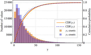
- Output distribution compatible with real data: using simulations from [20], obtained on a sample of approximately \(1.53\times10^5\) values, we imposed that the range and distribution of \(y\) be similar to those observed in real datasets. A comparison between the CDF of the final test function (Eq. 2.8) and the CDF of the data from [20] is shown in Figure 3.
- T2.3: Testing
During this stage of the project, the development of the T3ST code has been completed. T3ST is a numerical FORTRAN code implementing the mathematical description of charged-particle dynamics in tokamak configurations, as presented earlier. Moreover, the code can include axisymmetric equilibrium magnetic fields at different levels of description (circular model, Solov’ev model, or equilibria reconstructed from experimental data). On top of this equilibrium field, Coulomb collisions and electrostatic turbulent fields are superimposed. The latter are modelled statistically using the principle of statistical representability, through random fields with predefined statistical characteristics.
Charged particles are dynamically followed in this electromagnetic environment using a numerical solver for the equations of motion, based on a 4th-order Runge–Kutta scheme. Once the particle trajectories are obtained, radial transport is estimated at the level of the convection and radial diffusion coefficients, computed in the usual way from the average position and dispersion of the trajectories:
$$ V_r(t\,|\,x)=\frac{d\langle X(t\,|\,x)\rangle}{dt}, \qquad D_r(t\,|\,x)=\frac12\frac{d}{dt}\left(\langle X(t\,|\,x)^2\rangle - \langle X(t\,|\,x)\rangle^2\right). $$
At the time of the funding proposal, the T3ST code (although unnamed at the time) was already about 90% complete and had been used in several theoretical investigations. As of this report, T3ST has undergone several improvements, detailed below.
Refinement of collision routines
Fokker–Planck operators for Coulomb collisions, $$ C[f,f_s] = -\partial_z\left(K_z f - D_{zz'}\,\partial_{z'} f\right), $$ have been previously derived in the literature for gyrokinetic coordinates [15].
Since T3ST follows particle trajectories $\{X(t), v_\parallel(t), \mu(t)\}$, we must describe collisions at this level. Collisions modify the gyroscopic dynamics, turning the deterministic ODE system into a set of stochastic differential equations (SDEs):
$$ d\mathbf{X} = \sqrt{2D_c\,(I-\mathbf{b}\otimes\mathbf{b})}\,d\mathbf{W}_X, $$
$$ dv_\parallel = v_\parallel\!\left[ -\nu + \left(\frac{2D_\parallel - D_\perp}{v^2} + \frac{\partial D_\parallel}{\partial v}\right) \right] dt + \Sigma_{v_\parallel,v_\parallel} dW_{v_\parallel} + \Sigma_{v_\parallel,\mu} dW_\mu, $$
$$ d\mu = \mu\!\left[ -2\nu + mE\!\left( v_\parallel \frac{\partial D_\parallel}{\partial v} + \frac{3(D_\parallel-D_\perp)(\mu B + 2E D_\perp)}{\mu B} \right) \right] dt + \Sigma_{\mu,v_\parallel} dW_{v_\parallel} + \Sigma_{\mu,\mu} dW_\mu, $$
where $dW_i$ are independent Wiener processes with zero mean.
Besides the full Coulomb operator, T3ST also implements a simplified Lorentz operator, useful especially for electron transport and providing a reasonable approximation for ions in coronal equilibrium with the background plasma. This formulation describes the evolution of the pitch angle $\lambda = v_\parallel/v$, where $v=\sqrt{v_\parallel^2 + v_\perp^2}$, and the kinetic energy $E_k$:
$$ \lambda(t+\Delta t) = \lambda(t) - \nu_d \lambda(t)\Delta t + \sigma\,(1-\lambda(t)^2)\nu_d\Delta t, \qquad (?) $$
$$ E_k(t+\Delta t) = E_k(t) - 2\nu_e\Delta t\, E_k(t) T \left(\frac{1}{T} - \frac{3}{2}\frac{E_k}{T} - \frac{d\ln\nu_e}{dE_k}\right) + 2\sigma\sqrt{\nu_e \Delta t\, E_k(t) T }. \qquad (?) $$
Here $\sigma=\pm1$ is a random sign chosen independently for each particle at each step. $T$ is the background plasma temperature, and $\nu_d$ and $\nu_e$ are the deflection and energy-transfer collision frequencies:
$$ \nu_d(v)= \frac{2\ln\Lambda\, n_i (Z_{\text{eff}} Z e^2)^2}{\pi\epsilon_0^2 m^2 v_{\text{th}}^3} \frac{\Phi(v)-\Psi(v)}{v^3}, \qquad (?) $$
$$ \nu_e(v)= \frac{\ln\Lambda\, n_i (Z_{\text{eff}} Z e^2)^2}{4\pi\epsilon_0^2 m^2 v_{\text{th}}^3} \frac{\Psi(v)}{v^3}. \qquad (28) $$
with $\ln\Lambda = 17$ the Coulomb logarithm, and the functions:
$$ \Phi(v) = \operatorname{erf}(v), \qquad (?) $$
$$ \Psi(v) = \frac{1}{2v^2}\big[\Phi(v) - v\,\Phi'(v)\big]. \qquad (?) $$
Equations (??) preserve both the isotropy of the pitch-angle distribution and the Maxwell–Boltzmann energy distribution: $$ P(\lambda, t+\Delta t) = P(\lambda). $$
Refinement of additional routines
Using real magnetic equilibria from preprocessed G-EQDSK files requires interpolation procedures to evaluate magnetic quantities along particle trajectories, which evolve in a Lagrangian manner, not on a fixed grid. Moreover, for initializing particle positions at $t=0$, most scenarios in T3ST require a uniform distribution of particles along a chosen magnetic flux surface. The previous implementation contained minor technical issues that introduced small spurious effects in the transport coefficients.
Within task T2.1, we identified, corrected, and improved the Fortran routine responsible for initializing particles on magnetic flux surfaces in experimentally reconstructed equilibria. The new routines are: psisurf_efit3, extract_contour_zero, order_points_by_angle, and interp_point_along_contour.
The routine psisurf_efit3 reconstructs magnetic flux surfaces from EFIT data and returns a representative point on each surface for a given parallel velocity $v_\parallel$. It reconstructs the poloidal flux $\psi(R,Z)$ and associated quantities $(F,\partial_R\psi,\partial_Z\psi)$ on a regular $(R,Z)$ grid, computes the magnetic field magnitude, and forms a modified scalar field:
$$ \phi(R,Z) = \psi - \psi_0 - K\,\frac{F}{|B|}\,V_p(k). $$
For each $v_\parallel$, the routine identifies the zero contour of $\phi(R,Z)$ — corresponding to the desired flux surface — using the auxiliary procedure extract_contour_zero, which locates sign changes of $\phi$ along cell edges and interpolates zero-crossing positions. A random point from this contour is selected as the particle position $(X(k), Y(k))$. If no valid contour is found, a fallback central value is used. The loop over all particles is parallelized with OpenMP.
Aggressive parallelization strategies
The most important improvement in T3ST in 2025 concerns program structure, leading to a roughly order-of-magnitude speed-up. This allows numerical simulations with satisfactory resolution (e.g., $N_p=10^6$, $N_c=200$, $N_t=1000$) on available hardware (~96 threads) in about one minute.
In previous versions, the most expensive computation was the evaluation of turbulent fields (and their derivatives), because it scaled as $\mathcal{O}(N_p N_c)$, where $N_p$ is the number of particles and $N_c$ the number of Fourier modes. By comparison, all other components scale as $\mathcal{O}(N_p)$. Thus, the earlier paradigm computed all quantities in series with vectorized operations, while only the turbulent components were parallelized.

Within WP2, we explored a complementary configuration: parallelizing all operations over the particles ($N_p$). Surprisingly, this approach led to a substantial performance improvement. A representative plot of computation time vs. particle number is shown in Figure 1 (log scale), where comparison between the old and new parallelization models reveals a speed-up of approximately a factor $\sim 11$.
In recent years, the Wolfram Mathematica platform [24] has integrated an extensive set of tools for the construction, training, and analysis of neural networks, collectively referred to as the Wolfram Language Neural Net Framework. This framework is complemented by a large collection of pre-trained models available through the Wolfram Neural Net Repository, as well as associated packages. These tools provide native support and advanced functionality for defining network architectures, representing neural models, training and deploying them, and selecting optimization procedures, loss functions, and regularization techniques—either predefined or user-customizable.
In the context of the objectives of Task T1.3, these capabilities are particularly well aligned with our requirements. They significantly reduce the time needed to develop the underlying software infrastructure and allow us to focus primarily on the physical problem of predicting turbulent transport. During the recent work period, we employed these libraries to develop and test a complete set of machine-learning tools adapted to data generated by numerical simulations performed with the T3ST code.
In order to evaluate different neural-network methods and training options prior to generating the actual database, we introduced an intermediate step in which several architectures, models, and training strategies were tested using a test function with dimensionality varying between 1 and 25 variables. This step is crucial because the generation of the real database is computationally expensive.
By contrast, using a test function—whose training dataset can be expanded arbitrarily—allows us to study sampling strategies, obtain an approximate estimate of the minimum required training-set size, compare different optimization and training methods, and explore the possibility of iterative neural-network training. This preliminary information provides practical guidance for generating the real database, avoiding oversizing and excessive computational costs.
Characteristics of the test function
When selecting the test function (defined as \(f(\mathbf{X}) = y\), where the pairs \(\mathbf{X} \rightarrow y\) form the dataset), we imposed the following criteria to preserve similarity with the behavior of the real asymptotic diffusion:
Consequently, under the conditions listed above, the final form of the test function is:
where \(i\in\overline{(1,N)}\) indexes the components of the input vector \(\mathbf{X}\); \(\alpha_i\in(0,1]\), \(\beta_i\in[0,5]\), \(\gamma_i\in[1.5,5.5]\) are scalar coefficients; and \(P_1^{(i)}(\mathbf{X})\), \(P_2^{(i)}(\mathbf{X})\) are random combinations of sums of terms of the form
The procedure defined by Eq. (2.8) generates sufficiently complex terms to reproduce variations similar to those observed in the real physical model, while maintaining relatively simple one-dimensional dependencies (continuous, smooth, and approximately monotonic), in agreement with observations from [20,21,22]. The sum of these terms yields a strictly positive output \(y>0\), with a distribution comparable to that of real simulations.
For the preliminary tests, the training dataset was sampled over the interval \([2.0,\,8.5]\), which approximately corresponds to the relevant ranges of the scaled parameters in the real model. Since the real data contain a small level of Gaussian noise (<10%), the same noise level was introduced into the test-function data to preserve representational fidelity.
Data normalization
To improve neural-network accuracy and accelerate training, both inputs and outputs are normalized before being fed into the network. This step is required when activation functions such as sigmoid or \(\tanh\) are used, as their ranges are strictly bounded around 0 and \(\pm1\).
Although standardization to zero mean and unit variance is commonly used, for the present dataset this procedure leaves a large fraction of output values outside the active region of the \(\tanh\) function. Therefore, scaling is performed to the interval \([-1,1]\) using the linear transformation:
where \(X\) denotes either the input components \(X_i\) or the output \(y\). This normalization ensures that the network operates in the nonlinear regime of the activation function and that outputs remain bounded within \(\pm1\).
Mitigation of overfitting
Overfitting occurs when a neural network learns the fine details and noise of the training data rather than extracting generalizable structures. As a result, the model effectively memorizes the training examples and loses predictive capability on unseen data.
Wolfram Mathematica [24] provides several efficient mechanisms to prevent overfitting, two of which
are particularly relevant here. The first involves the use of a validation dataset via the
ValidationSet option. After each training round, the network is evaluated on this dataset, and
Wolfram automatically selects the intermediate network state that minimizes the validation loss rather
than the training loss.
The second method is early stopping, activated through the TrainingStoppingCriterion option in
combination with ValidationSet. If the validation loss starts to increase—indicating the onset
of memorization—the training process is automatically halted. Together, these two mechanisms provide
robust control of overfitting by continuously monitoring validation performance and preventing excessive
model complexity.
Training an ensemble of neural networks
Due to the random initialization of weights and biases, the final trained configurations differ from one neural network to another. Although training should ideally converge toward a region close to the global minimum of the loss function, the optimization trajectories differ, and convergence to the global minimum cannot be guaranteed. As a result, individual networks produce slightly different predictions.
A solution to this issue is to train multiple networks and define the final prediction as the average of their individual predictions—an approach known as a neural-network ensemble [23]. The effectiveness of this method follows from the Central Limit Theorem: individual errors and biases tend to cancel out, and the ensemble average converges toward the true function value.
Code fragments used during the testing phase
Figure 4 shows a code fragment illustrating the generation of the test function, the training and
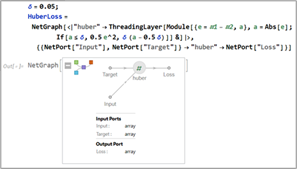
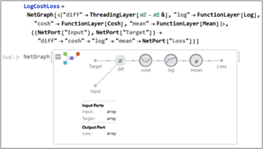
validation datasets, and their scaling. Figures 5a–b present code fragments in which two loss functions
are constructed using the NetGraph function.
Defining the difference between neural-network predictions and true values as \(\varepsilon = y - \hat{y}\), the first loss function is the Huber loss:
where \(\delta\) is a hyperparameter chosen based on the noise level in the training data. The second loss function is the Log-Cosh loss:
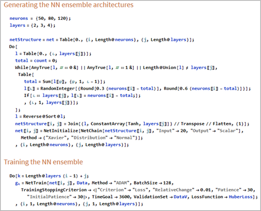
Finally, Figure 6 presents a code fragment illustrating the generation of network architectures and the training of the neural-network ensemble using the Huber loss function and overfitting-mitigation techniques.
The development of the T3ST code took place over several years and culminated in the present project, during which the last refinements and improvements to the numerical tool were made. Consequently, the code has gone through an extensive sequence of testing stages, targeting both specific implementations and large-scale results.
In this report we restrict ourselves to presenting three examples relevant to transport aspects. The first two refer to purely neoclassical dynamics (in the absence of turbulence) at the microscopic level, while the third test integrates almost all components of the code simultaneously.
We begin by checking whether the neoclassical trajectories (without turbulence) satisfy the minimal requirements regarding the correctness of their topology. For this purpose we analyse (Figure 2) two randomly chosen trajectories, which illustrate both the characteristic geometry of passing particles and that of “banana” orbits, both properly closed in the poloidal projection, in a circular configuration.
The second test targets the quantitative aspect of the trajectories. To this end, we generate a set of particles with a Maxwell–Boltzmann energy distribution, with pitch angles uniformly distributed in the interval \((0, 2\pi]\), and their initial positions placed on a magnetic surface corresponding to a circular equilibrium (thus at a fixed radius, but uniformly distributed in the toroidal and poloidal angles).
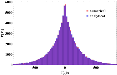
Using the circular model (see equation ??), it can be shown that a very good approximation of the radial velocity is provided by the analytical expression
In Figure 3 we present the distribution of radial velocities obtained in the analysed scenario, both from the analytical formula mentioned above and from the simulations carried out with the T3ST code. The two distributions are seen to coincide almost perfectly, which constitutes a solid validation of the way in which the guiding-centre drifts are calculated (at least in the non-turbulent regime).
The last and probably most important test is illustrated in Figure 4. The scenario considered is the following: hydrogen ions are distributed according to a Maxwell–Boltzmann distribution in energy and uniformly in pitch angle. The spatial distribution is chosen such that all particles possess approximately the same toroidal momentum, in direct connection with the new routine developed during stage T1.2:
This initial distribution is very close to a gyrokinetic equilibrium (as opposed to a distribution uniform on a magnetic surface). We therefore expect that particles distributed in this way will exhibit only a short transient phase, after which they will rapidly settle into a genuine equilibrium state, characterised by vanishing transport coefficients.
In this scenario, after reaching the quasi-equilibrium state, turbulence is initialised and the particle dynamics are then followed further. It can be shown—although the analysis is beyond the scope of this paper—that, under the given conditions, the quasilinear approximation of the diffusion (valid for short times immediately after the onset of turbulence) can be written as
The complexity of this test is also visible in the analytical formula inspired by quasilinear theory. It includes the turbulence intensity, the geometric effects associated with toroidicity, the spectrum of poloidal wavenumbers, as well as finite Larmor radius effects, which enter directly into the statistical average through the Bessel function \(J_0\).
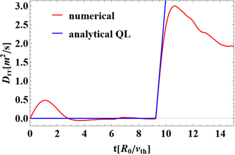
In Figure 5 the results of this complex test are presented. As expected, in the absence of turbulence, the transient dynamics are short and the system rapidly converges towards a state without transport. This state is then “excited” by turbulence (around time \(t \approx 9\)), and the initial slope of the evolution is predicted with very high accuracy by the quasilinear result at short times.
Testing the machine-learning tools
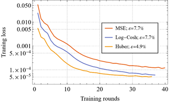
We initiated the testing phase of the machine-learning tools described in Tasks T1.3 and T2.2 by evaluating the convergence speed of the two loss functions defined in Eqs. (2.10) and (2.11), in comparison with the standard mean squared error (MSE). For this purpose, we trained three identical neural networks, each with two hidden layers containing 50 and 30 neurons, respectively, using Xavier normal initialization and the ADAM optimization algorithm.
The training set consisted of \(10^5\) samples. Automatic stopping of the training process was implemented using the criterion that the relative variation of the validation error must remain below 1% for at least 15 consecutive epochs. Figure 9 shows the evolution of the three loss functions during training. In the legend, \(\varepsilon\) denotes the relative error between the predictions of the neural networks and the true values \(y\) in the validation set:
The results show that the Huber loss function leads to both faster convergence and more accurate predictions. Consequently, the Huber loss function is adopted for all subsequent tests.
Prediction error, test-function dimensionality, and ensemble model selection
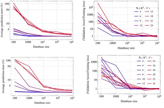
We investigated the influence of the dimensionality of the test function and the size of the dataset on model performance. Eight test functions with dimensionalities between 2 and 24 variables were used, along with datasets ranging from \(10^2\) to \(10^6\) samples (five values). In total, 40 neural networks were trained using the same architecture: two hidden layers with 80 and 40 neurons.
All other training details were identical to those described in the previous subsection. The analysis begins with the evolution of the error \(\varepsilon\) (Eq. 2.15) as a function of the training-set size (Figures 10a–b). For all eight test functions, the error saturates at approximately \(10^5\) training samples, independently of the number of variables.
We also examined the possibility of overfitting. Figure 10b shows the ratio between validation error and training error as a function of dataset size. This ratio approaches unity for datasets larger than \(\sim 10^5\) samples, indicating the absence of overfitting and confirming that a database of order \(10^5\) is sufficient.
Finally, we compared these results with those obtained using a deeper architecture featuring four hidden layers and a total of 500 neurons. Sixty such networks were trained. Figures 10c–d show that, although the number of parameters increases from approximately 5,000 to about 54,500, the performance does not improve significantly: neither the prediction error, nor its dependence on dataset size, nor the training-to-validation error ratio exhibits meaningful gains.
Based on these results, we selected an ensemble composed of nine neural networks for subsequent tests, corresponding to combinations of 2, 3, and 4 hidden layers with 50, 80, and 120 neurons.
Recurrent training of the neural-network ensemble
We continued the testing phase by analyzing the feasibility of recurrent neural-network training, a technique designed to reduce the initial computational cost by starting from a small dataset. This approach is particularly advantageous when data originate from numerical simulations rather than from an analytical test function.
The method consists of using a neural-network ensemble to evaluate the variance of predictions on the validation set, selecting points with high variance or large errors. To determine which of the 20 input parameters vary significantly near each point, we compute the gradient of the prediction with respect to each parameter and retain only those variables associated with significant gradients. Based on this information, a new training set is generated and the ensemble is retrained.
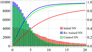
We tested this approach using the ensemble defined in the previous subsection, starting from an initial dataset of \(10^3\) samples. After the initial training, two additional datasets of \(10^3\) samples each were generated: one using the adaptive procedure and a control dataset generated uniformly. The networks were retrained separately on these two datasets.
Performance was evaluated by comparing the predictions of the three ensembles on a uniformly sampled test set of \(10^5\) examples. Figure 11 shows the distributions of the percentage errors defined in Eq. (2.15), as well as their cumulative distribution functions.
The results demonstrate a clear improvement for the adaptively retrained model: approximately 94% of the errors are below 10%, compared to about 89% for the control model and roughly 64% for the initially trained ensemble.
We therefore conclude that adaptive retraining represents a viable strategy for reducing the total computational cost, even when accounting for the additional expense of retraining. This approach enables the use of a relatively small initial dataset, which can subsequently be expanded in an informed and efficient manner during the training process.
O3 (WP3) – The construction of the database: extensive simulations
Deliverable: Database, trained and tested machine learning tools
...O4 (WP4) – Predictions and physical mechanisms
Deliverable: Characterization of transport mechanisms
...